Temporal Behaviour of Turbulence

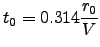
A model for the time-dependence of the phase fluctuations can be derived from the spatial fluctuations under the assumption of ``frozen turbulence'', that is to say that the turbulent cells are blown past the observer faster than the cells themselves evolve. Observational evidence for the validity of this hypothesis has been obtained by Caccia, Azouit & Vernin (1987), although only for cells of air with characteristic sizes of a few cm. Under this assumption, the temporal phase structure function will have the form

$$D_{t,\varphi}(t)\equiv\left\langle [\varphi(t')-\varphi (t'+t)]^{2}\right\rangle= (\frac{t}{t_0})^{5/3}$$ (2.9)

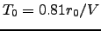
where $\varphi(t)$ is the phase perturbation at a given point on the wavefront at time $t$. This equation serves to define a 'coherence time' $t_0$ (Buscher 1988) which is related to $r_0$ and the windspeed $V$ by the equation :

$$t_0=0.314\frac{r_0}{V}$$ (2.10)

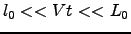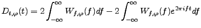
It should be noted that no single definition of the coherence time has been adopted by the optical community. Colavita, Shao & Staelin (1987) define a coherence time $T_0$ such that $T_0=0.81r_0/V$. As in the spatial case, equation 2.10 is valid only for $l_0 << Vt << L_0$. Where $l_0$ and $L_0$ is the inner and outer scale of turbulence respectively. Also the velocity $V$ is given by the equation :

$$V=\Bigg[\frac{\int_0^\infty C_n^2(h)\cdot V(h)^{5/3}dh}{\int_ 0^\infty C_n^2(h)dh}\Bigg]^{3/5}$$ (2.11)

Where $C_n^2(h)$ is the vertical profiles of the turbulence and $h$ the height from the ground.

Finally, we can define the relationship between the temporal power spectrum $W_{f,\varphi }$ and the temporal structure function of the phase perturbations via a Fourier transform :

$$D_{t,\varphi}(t)=2\int_{-\infty}^{\infty}W_{f,\varphi}(f)df-2\int_{-\infty}^{\infty}W_{f,\varphi}(f)e^{2\pi ift}df$$ (2.12)

This gives for the structure function of equation 2.9 a power spectrum :

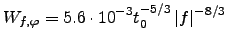$$W_{f,\varphi}=5.6\cdot 10^{-3}t_0^{-5/3}\left\vert f\right\vert^{-8/3}$$ (2.13)

In the above discussions it has been assumed that there is a single layer of turbulence being blown past the observer. In fact there is a large body of experimental evidence showing that there are many layers of turbulence at difference heights contributing to the seeing, each a few metres thick each moving with a different speed and direction, and each with its own outer scale. The properties of the seeing affecting a star observed at ground level will be an average of the properties of these layers, weighted by the strength of the refractive-index fluctuations in each layer. Thus, for example, $V$ in equation 2.10 will be an `average windspeed', rather than the speed of any particular layer. Here something must be mentioned about the effects of dome seeing. The steep temperature gradients formed by the mixing of warm air in the dome (produced by instruments and machinery) and colder air outside can produce very strong refractive index effects. Any turbulent cells inside the dome will be driven primarily by convection and so will not conform to the `frozen turbulence' assumption. It is also likely that these will not be described by Kolmogorov statistics, i.e. the turbulence is not `fully developed'. As you can understand coherence time $t_0$ is very important for adaptive optics systems, since it is the minimum time that corrections must be done.