ESO-DIMM

The ESO-DIMM method in order to produce the two images in the focal plane, uses a prism in one of the Hartmann hole to deverse light. Below is the theory of the ESO-DIMM.

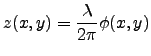
The wavefront corrugation $z(x,y)$ is proportional to the wavefront phase error $\phi(x, y)$ :

$$z(x,y)=\frac{\lambda}{2\pi}\phi (x,y)$$ (3.1)

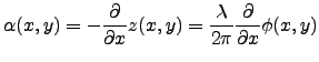
Since light rays are normal to the wavefront surface, the component $\alpha$ of the angle-of-arrival fluctuation in the $x$ direction is given by :

$$\alpha (x,y)=- \ensuremath{\frac{\partial}{\partial x}}z(x,y)=\frac{\lambda}{2\pi} \ensuremath{\frac{\partial}{\partial x}}\phi (x,y)$$ (3.2)

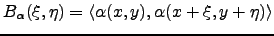
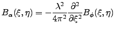
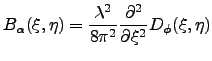
Hence, the covariance of the angle-of-arrival fluctuation is :

$$B_\alpha (\xi ,\eta)=\left\langle \alpha (x,y),\alpha (x+\xi,y+\eta)\right\rangle$$ (3.3)

is related to the covariance $B_\phi (\xi ,\eta)$ of the phase fluctuation by :

$$B_\alpha (\xi ,\eta)=-\frac{\lambda^2}{4\pi^2}\ensuremath{\frac{\partial^2}{\partial\xi^2}}B_\phi (\xi ,\eta)$$ (3.4)

and introducing the phase structure function :

$$D_\phi (\xi,\eta)=2\big[B_\phi (0,0)-B_\phi(\xi,\eta)\big]$$ (3.5)

and so it becomes :

$$B_\alpha (\xi ,\eta)=\frac{\lambda^2}{8\pi^2}\ensuremath{\frac{\partial^2}{\partial\xi^2}}D_\phi(\xi,\eta)$$ (3.6)

For Kolmogorov turbulence at the near-field approximation, the phase structure function is given by the widely used expression (2.3) :

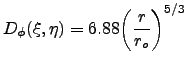$$D_\phi(\xi,\eta) = 6.88\bigg(\frac{r}{r_o}\bigg)^{5/3}$$ (3.7)

where 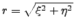$r=\sqrt{\xi^2+\eta^2}$ and $r_o$ is Fried's seeing parameter. Putting 3.7 into 3.6 gives :

$$B_\alpha(\xi,\eta)=0.145\lambda^2r_0^{-5/3}\bigg[(\xi^2+\eta^2)^{-1/6}-\frac{1}{3}\xi^2(\xi^2+\eta^2)^{-7/6}\bigg]$$ (3.8)

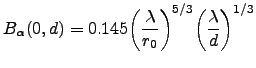
For $\eta=0$ we get the longitudinal covariance (in the direction of the tilt) as a function of the separation $\xi=d$ :

$$B_\alpha(d,0)=0.097\bigg(\frac{\lambda}{r_0}\bigg)^{5/3}\bigg(\frac{\lambda}{d}\bigg)^{1/3}$$ (3.9)

For $\xi=0$, we get the lateral or transverse covariance (in a direction perpendicular to the tilt) as a function of the separation $\eta=d$ :

$$B_\alpha(0,d)=0.145\bigg(\frac{\lambda}{r_0}\bigg)^{5/3}\bigg(\frac{\lambda}{d}\bigg)^{1/3}$$ (3.10)

The transverse covariance is exactly 1.5 times larger than the longitudinal covariance and both decrease as the $-1/3$ power of the separation. This was well confirmed experimentally by Borgnino et al. (1978). These expressions are valid only within the inertial range of the Kolmogorov spectrum. The divergence at the origin is clearly not physical. In practice, the value at the origin is limited by aperture averaging and is given by the expression for the variance of image motion derived by Fried (1965, 1975), and Tatarski (1971), (within a factor of two since we consider motion in one direction only) :

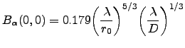$$B_\alpha(0,0)=0.179\bigg(\frac{\lambda}{r_0}\bigg)^{5/3}\bigg(\frac{\lambda}{D}\bigg)^{1/3}$$ (3.11)

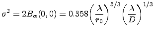
where D is the diameter of the apertures through which tilts are measured. Because of the slow decrease of the covariance as the $-1/3$ power of the distanced in 3.9 and 3.10, aperture averaging does not noticeably modify the covariance function as soon as the distance exceeds twice the aperture diameter, as shown below. The variance $\sigma^2(d)$ of the differential image motion observed over a distance $d$ is given by :

$$\sigma^2(d)=2\big[B(0)-B(d)\big]$$ (3.12)

Putting 3.9 and 3.11 into 3.12 gives an approximate expression for the variance $\sigma_l^2$ of the differential longitudinal motion for $d\geq2D$ :

$$\sigma_l^2=2\lambda^2r_0^{-5/3}\big[0.179D^{-1/3}-0.0968d^{-1/3}\big]$$ (3.13)

whereas putting 3.10 and 3.11 into 3.12 gives an approximate expression for the variance $\sigma_t^2$, of the differential transverse motion for $d\geq2D$ :

$$\sigma_l^2=2\lambda^2r_0^{-5/3}\big[0.179D^{-1/3}-0.145d^{-1/3}\big]$$ (3.14)

These variances can be expressed in terms of the total variance for $2$-dimensional motion through a single aperture of diameter $D$ :

$$\sigma^2=2B_\alpha(0,0)=0.358\bigg(\frac{\lambda}{r_0}\bigg)^{5/3}\bigg(\frac{\lambda}{D}\bigg)^{1/3}$$ (3.15)

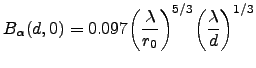
Putting 3.15 into 3.13 and 3.14 with $S=d/D$ gives :

$$\sigma_l^2=\big[1-0.541S^{-1/3}\big]\sigma^2$$

$$\sigma_t^2=\big[1-0.811S^{-1/3}\big]\sigma^2$$

The above equations are the basis of the DIMM method.